What Is Atomic Force Microscopy (AFM)?

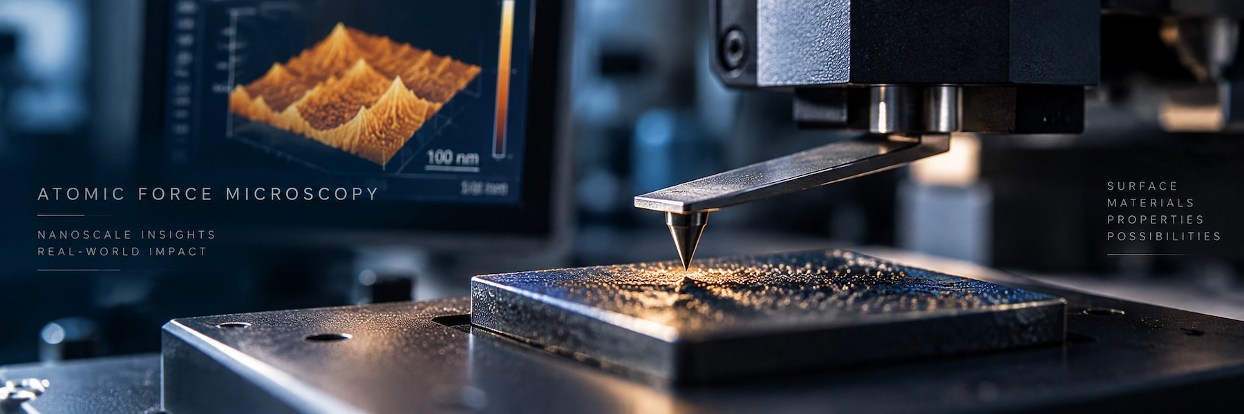
If an atomic force microscope does not actually “see” a surface, what exactly is it measuring?

Short Answer

Atomic force microscopy (AFM) is a scanning probe microscopy technique used to characterize surfaces at the nanoscale by measuring interactions between a sharp probe and a sample. Rather than directly “seeing” nanoscale objects, an AFM converts tip–sample interactions into quantitative information about surface topography, morphology, height, and roughness. With the appropriate AFM mode, probe, and instrument configuration, the same platform can also investigate local mechanical, electrical, magnetic, and electromechanical properties.

The key idea is simple but often overlooked:

An AFM image is not just a picture of a surface—it is the result of a controlled physical interaction between a probe, a sample, and a measurement system.

Understanding that interaction is the key to understanding how AFM works, what AFM actually measures, what determines AFM resolution, how to choose an AFM mode and probe, why AFM artifacts occur, and whether AFM is the right characterization technique for an experiment.

Understanding Atomic Force Microscopy

Atomic force microscopy is a surface-characterization technique in the scanning probe microscopy family. It uses a nanoscale probe attached to a flexible cantilever to scan a sample while monitoring interactions between the probe tip and the surface.

The atomic force microscope was introduced in 1986 by Gerd Binnig, Calvin Quate, and Christoph Gerber. Their original instrument extended scanning-probe concepts beyond the tunneling-current requirement of scanning tunneling microscopy (STM), making force-based surface characterization possible for insulating as well as conducting materials.

Modern AFM has developed far beyond its original role. It is now better understood as a nanoscale measurement platform rather than a single imaging technique.

At its most basic, AFM provides information about surface topography. With specialized probes, operating modes, electronics, and environmental controls, AFM platforms can also investigate properties including adhesion, friction, stiffness and other mechanical responses, electrical current, surface potential, magnetic interactions, and electromechanical behavior.

However, these are not universal capabilities of every atomic force microscope.

AFM as a technique must be distinguished from the capabilities of a specific AFM instrument.

---

Recommended AFM Books:

Best Overall: Eaton & West — Atomic Force Microscopy ·

Best for Practical AFM: Greg Haugstad — Atomic Force Microscopy ·

Best for Researchers: Bert Voigtländer — Atomic Force Microscopy

Affiliate disclosure: As an Amazon Associate I earn from qualifying purchases.

---

What is AFM mainly used for?

AFM is primarily used when researchers need localized information about a surface at micro- to nanoscale dimensions, particularly surface topography, roughness, morphology, feature height, and nanoscale surface structure.

Specialized AFM methods expand that role into local property mapping.

What Does an Atomic Force Microscope Actually Measure?

An atomic force microscope does not directly record a conventional optical image of the surface. Instead, it measures a physical response produced by interactions between the probe and the sample.

A typical AFM probe consists of a sharp tip positioned at or near the end of a microscopic cantilever. As the probe moves across the sample, tip–sample interactions alter the cantilever’s behavior.

Depending on the AFM mode, the instrument may monitor quantities such as:

• cantilever deflection;
• oscillation amplitude;
• oscillation phase;
• resonance frequency or frequency shift;
• force;
• electrical current;
• electrical potential-related signals;
• other interaction-dependent observables.

A feedback controller uses the relevant signal to maintain a defined imaging or measurement condition while the probe scans the surface.

For conventional topographic imaging, the vertical movement required to maintain that interaction condition provides information used to reconstruct the surface topography.

The basic measurement chain can therefore be represented as:

Sample → Tip–Sample Interaction → Cantilever Response → Detection → Feedback → Scanner Motion → Recorded Data → AFM Image or Property Map

This chain explains an essential principle of AFM:

The measured AFM dataset contains information about both the sample and the measurement process.

Probe geometry, probe condition, tip–sample forces, scanner behavior, feedback parameters, vibration, thermal drift, environment, sampling, and data processing can all influence the final result.

Does AFM directly see atoms?

No—not in the same sense that a conventional microscope forms an image using light or electrons.

AFM detects interactions between a probe and a sample and reconstructs spatial information from those measurements.

Under specialized experimental conditions, particular AFM implementations can resolve atomic-scale structure, but this should not be generalized to routine AFM imaging.

How Does Atomic Force Microscopy Work?

The simplest mental model is to imagine an extremely small stylus tracing a landscape.

As the AFM tip moves over hills, valleys, particles, grains, terraces, steps, and other features, its interaction with the surface changes. The microscope detects these changes and adjusts the relative probe–sample position.

Real AFM operation is considerably more sophisticated.

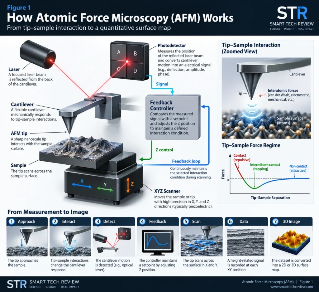
1. The AFM tip approaches the sample. A sharp probe is positioned close to, or in controlled contact with, the sample.
2. Tip–sample interactions affect the cantilever. Forces or force gradients between the tip and sample alter the cantilever’s deflection or dynamic behavior.
3. The cantilever response is detected. Many AFMs use an optical lever system in which a laser is reflected from the back of the cantilever onto a position-sensitive photodetector. Other detection architectures also exist.
4. The probe scans across the surface. A precision scanner controls relative movement between the probe and sample in X, Y, and Z.
5. A feedback loop maintains the measurement condition. The controller compares the measured signal with a selected setpoint and adjusts probe–sample separation as necessary.
6. The instrument constructs a dataset. Scanner position and interaction-dependent signals are converted into topographic images or other property maps.

Figure 1 — How Atomic Force Microscopy Works
Diagram showing the optical lever detection system, cantilever, tip–sample interaction, XYZ scanner, photodetector, and closed feedback loop.

How does AFM create a 3D surface image?

For topographic imaging, AFM records height-related information across XY positions on the sample.

The resulting dataset can be displayed as a three-dimensional representation of the surface. However, the rendered image should not be interpreted as a perfect geometrical replica of the real surface because tip geometry, feedback behavior, drift, noise, sample deformation, and other effects can influence the measurement.

Main Components of an Atomic Force Microscope

An atomic force microscope consists of several closely integrated components that work together to control the tip–sample interaction, detect the probe response, scan the sample, and reconstruct measurement data.

AFM component	Main function
Probe	Carries the tip and interacts with the sample
Tip	Creates a highly localized tip–sample interaction
Cantilever	Mechanically responds to forces or force gradients
Detection system	Measures cantilever deflection or dynamic response
Laser	Used in many optical-lever AFMs to monitor cantilever motion
Photodetector	Detects changes in reflected laser position
XYZ scanner	Controls precise relative movement between sample and probe
Feedback controller	Maintains the selected interaction condition
Control electronics	Coordinate excitation, detection, scanning, and acquisition
Software	Controls measurements and processes AFM data
Isolation system	Reduces vibration, acoustic noise, and environmental disturbance

Why the AFM Probe Matters

The AFM probe is part of the measurement system, not simply a replaceable accessory. Its properties can directly influence what the instrument can measure and how accurately surface features are represented.

Tip radius, tip geometry, aspect ratio, cantilever spring constant, resonance frequency, coating, conductivity, magnetic properties, and probe material can all influence the suitability of a probe for a particular AFM experiment.

For example, tip geometry can affect the representation of narrow or steep surface features, while cantilever mechanical properties influence how the probe responds to tip–sample interactions. Specialized coatings or probe materials may also be required for electrical, magnetic, or other advanced AFM measurements.

From Tip–Sample Interaction to an AFM Image

One of the most important lessons in AFM is that the measured image is influenced by both the surface and the probe.

Why doesn’t an AFM image always show the exact surface shape?

Because the AFM tip has a finite geometry.

When a structure has dimensions comparable to the AFM probe, parts of the tip other than its ideal apex may interact with the feature during scanning. Consequently, measured structures can appear laterally broader than their actual dimensions.

This effect is commonly described as tip convolution.

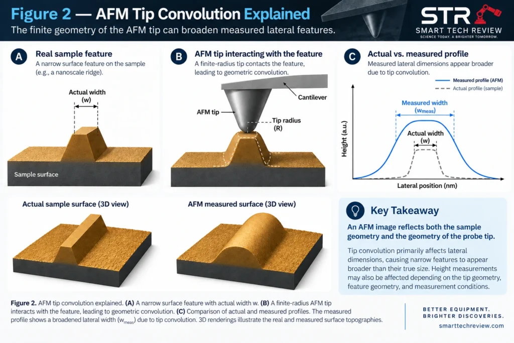
Height information can often be considerably less affected by simple geometrical broadening than lateral width, although height measurements have their own sources of uncertainty.

Probe wear and contamination can create additional problems. A contaminated or damaged tip may broaden structures or produce repeated or duplicated features that are not present on the real surface.

Never interpret an AFM image independently of probe condition, scan parameters, and measurement physics.

What Can AFM Measure?

Core topographic measurements

AFM can be used to investigate:

• surface topography;
• morphology;
• surface roughness;
• feature height;
• step height;
• grains and grain structure;
• particles and nanostructures;
• terraces;
• surface texture;
• local surface defects.

AFM can also function as a quantitative metrology tool when calibration, traceability, measurement conditions, and uncertainty are properly controlled.

Specialized AFM measurements

Property	Example AFM approach
Surface topography	Contact or dynamic AFM
Surface roughness	Topographic AFM
Adhesion	Force spectroscopy / force mapping
Mechanical response	Force mapping / nanomechanical methods
Friction	Friction or lateral-force microscopy
Electrical current	Conductive AFM
Surface potential	Kelvin probe force microscopy
Electromechanical response	Piezoresponse force microscopy
Magnetic interactions	Magnetic force microscopy
Molecular forces	Force spectroscopy

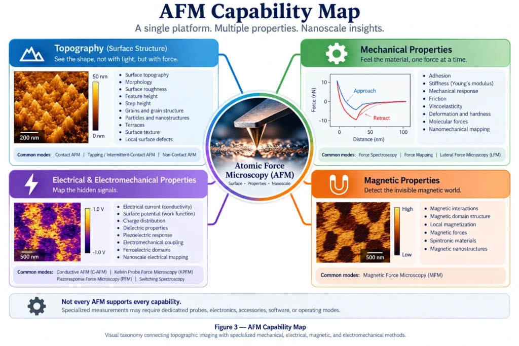
Can every AFM measure electrical or magnetic properties?

No.

These measurements normally require specialized probes, electronics, accessories, software, or operating modes.

Therefore:

AFM → technique

is not equivalent to:

AFM instrument → every AFM capability

What Are the Main Atomic Force Microscopy (AFM) Modes?

The three classical AFM interaction regimes are:

• Contact AFM
• Tapping or intermittent-contact AFM
• Non-contact AFM

The main difference between these AFM modes is how the probe interacts with the sample during scanning. This interaction influences image quality, forces applied to the sample, tip wear, and suitability for different materials.

Contact Mode AFM

In contact mode AFM, the probe remains in continuous mechanical contact with the sample while scanning.

Contact mode can provide excellent topographic data for appropriate samples. However, continuous contact also produces lateral forces that may deform soft materials, move weakly attached particles, accelerate tip wear, or damage delicate structures.

Tapping or Intermittent-Contact AFM

In tapping or intermittent-contact AFM, the cantilever oscillates and periodically interacts with the sample rather than maintaining continuous contact.

Reduced lateral loading is one reason dynamic AFM approaches are commonly used for polymers, nanostructures, biological materials, and other samples susceptible to lateral forces.

Terminology varies among manufacturers and AFM communities. Therefore, terms such as tapping, intermittent contact, AC mode, and specific commercial implementations should not automatically be assumed to describe identical feedback schemes.

Non-Contact AFM

In non-contact AFM, an oscillating probe interacts with the surface without intentional intermittent mechanical contact.

High-performance non-contact AFM can achieve atomic-scale characterization under specialized conditions, but stable operation depends strongly on instrumentation, environment, and measurement conditions.

Which AFM Mode Should I Use?

There is no universally best AFM mode. The appropriate mode depends on the sample, the property being investigated, the acceptable level of tip–sample interaction, the measurement environment, and the capabilities of the instrument.

A useful decision chain is:

Sample → Property of Interest → Allowable Tip–Sample Interaction → Required Information → Environment → Instrument Capability

Advanced AFM Modes

Beyond conventional contact, intermittent-contact, and non-contact operation, AFM can be extended with specialized measurement modes to investigate local electrical, electromechanical, magnetic, and mechanical properties.

Conductive AFM (C-AFM)

Conductive AFM (C-AFM) combines topographic scanning with localized electrical-current measurement using a conductive probe and a suitable electrical configuration.

C-AFM can therefore provide spatially resolved information about variations in local electrical conduction while simultaneously acquiring surface topography.

Kelvin Probe Force Microscopy (KPFM)

Kelvin probe force microscopy (KPFM) measures electrostatic potential-related contrast and is commonly used to investigate contact potential difference and infer local work-function-related variations under appropriate assumptions and calibration.

Because measured contrast can also depend on probe properties, environment, electrostatic interactions, and measurement configuration, KPFM data should be interpreted within the specific experimental context.

Piezoresponse Force Microscopy (PFM)

Piezoresponse force microscopy (PFM) detects electromechanical response produced by electrical excitation and is widely used in ferroelectric and piezoelectric materials research.

Interpretation requires care because measured signals can contain contributions beyond an ideal piezoelectric response.

Magnetic Force Microscopy (MFM)

Magnetic force microscopy (MFM) uses a magnetically responsive probe to investigate spatial variations in magnetic tip–sample interactions.

The resulting contrast reflects magnetic interactions under the selected measurement conditions and should not automatically be interpreted as a direct map of a single magnetic material property.

Force Spectroscopy

AFM force spectroscopy records force-related behavior during controlled probe approach, interaction, contact, and/or retraction.

Depending on the experiment and analysis model, force curves can provide information related to adhesion, mechanical response, molecular interactions, and other local tip–sample interactions.

Nanomechanical Mapping

Various AFM methods can spatially map local mechanical response.

Quantitative interpretation may require cantilever calibration, probe-geometry information, contact-mechanics assumptions, suitable material models, and well-controlled measurement conditions.

Does Every AFM Support These Advanced Modes?

No. Not every atomic force microscope supports every advanced AFM method.

Specialized measurements may require dedicated probes, sample holders, electronics, excitation or detection hardware, software, environmental control, or instrument-specific capabilities.

Some manufacturers also provide proprietary operating modes. These should be distinguished from broader measurement categories when comparing AFM capabilities across instruments.

What Is Atomic Force Microscopy (AFM) Resolution?

AFM resolution cannot be represented by a single universal number. It depends on the probe, sample, tip–sample interaction, instrument, environment, feedback conditions, and the type of measurement being performed.

Importantly, vertical resolution and lateral resolution are not the same thing and should be considered separately.

Can AFM Achieve Atomic Resolution?

Yes—under particular experimental conditions and with appropriate AFM implementations.

However, saying simply that “AFM has atomic resolution” is misleading.

Advanced dynamic AFM, particularly frequency-modulation AFM under carefully controlled conditions such as ultrahigh vacuum, has demonstrated atomic-scale and, in suitable systems, atomic-resolution imaging.

Routine AFM measurements should therefore not automatically be described as atomic-resolution measurements. The achievable resolution depends on the specific instrument, probe, sample, operating mode, environment, and measurement conditions.

Vertical Resolution

AFM can be extraordinarily sensitive to vertical displacement, which is one reason it is widely used for nanoscale surface-topography and step-height measurements.

Practical vertical performance nevertheless depends on factors such as detector noise, scanner noise, vibration, thermal stability and drift, feedback performance, environmental conditions, sample behavior, and instrument architecture.

Therefore, vertical resolution should not be treated as a fixed value that applies to every AFM experiment.

Lateral Resolution

Lateral resolution is strongly influenced by the AFM probe tip and its interaction with the sample.

Important factors include:

• tip radius;
• tip shape and aspect ratio;
• tip–sample interaction;
• sample geometry;
• sample deformation;
• feedback performance;
• signal-to-noise ratio;
• measurement conditions.

A finite tip radius can make narrow surface features appear broader than their true lateral dimensions—an effect known as tip convolution, illustrated in Figure 2.

What Determines AFM Resolution?

Instead of asking only “What is the resolution of an AFM?”, a more scientifically useful way to think about AFM resolution is:

AFM resolution = probe + sample + interaction + instrument + environment + feedback + measurement conditions

In other words, AFM resolution is a measurement-system property, not merely a single number printed on an instrument specification sheet.

AFM Probes and Cantilevers

Choosing the right AFM probe and cantilever is one of the most important experimental decisions in atomic force microscopy. The probe is not simply an accessory—it is part of the measurement system and can directly influence resolution, tip–sample interaction, image quality, and the reliability of the resulting data.

Relevant probe and cantilever properties include:

• tip radius;
• tip height;
• tip shape and aspect ratio;
• tip material;
• coating;
• electrical conductivity;
• magnetic properties or coating;
• cantilever spring constant;
• resonance frequency;
• cantilever geometry.

The appropriate combination depends on the sample, AFM mode, property of interest, expected feature geometry, environmental conditions, and acceptable tip–sample interaction.

No single AFM probe is optimal for every experiment.

Can the Wrong AFM Tip Change the Result?

Yes.

An unsuitable, contaminated, worn, or damaged AFM tip can reduce lateral resolution, distort measured feature dimensions, increase tip-convolution effects, damage or modify the sample, destabilize feedback, and generate artifacts that may be incorrectly interpreted as real surface structures.

For this reason, probe selection and probe condition should be considered part of AFM experimental design and data interpretation, rather than treated as an afterthought.

How Does Atomic Force Microscopy Measure Surface Roughness?

AFM measures surface roughness by recording spatially resolved height data across a defined scan area. Roughness parameters can then be calculated from the resulting topographic dataset after appropriate data processing.

Common AFM surface-roughness parameters include:

• Arithmetic mean roughness (Ra) — the mean absolute deviation of surface height from the reference or mean plane.
• Root-mean-square roughness (Rq or RMS roughness) — the root-mean-square deviation of surface height from the reference or mean plane.

However, an important principle is:

Surface roughness is not simply a material number independent of the measurement.

The reported AFM roughness value can depend on:

• scan size;
• scan location;
• pixel density and spatial sampling;
• probe geometry;
• probe condition;
• scanner behavior;
• image leveling or flattening;
• filtering;
• line correction;
• artifact identification and removal;
• the definition of the reported roughness parameter.

For this reason, a roughness value should ideally be interpreted together with the measurement area, acquisition conditions, data-processing procedure, and roughness metric used.

Can AFM Roughness Values From Two Papers Be Compared Directly?

Not necessarily.

A scientifically meaningful comparison should consider whether the studies used comparable scan sizes, sampling densities, probe characteristics, measurement conditions, preprocessing procedures, and roughness definitions.

Two studies can investigate nominally similar materials yet report different AFM roughness values partly because their measurement and data-processing conditions differ.

What Materials Can AFM Characterize?

Atomic force microscopy can characterize a wide range of materials and sample types, from hard inorganic surfaces to soft polymers and biological specimens.

Examples include:

• thin films and coatings;
• metals;
• ceramics;
• polymers;
• nanoparticles;
• nanowires;
• 2D materials;
• semiconductors;
• battery and energy materials;
• composites;
• biomaterials;
• biological specimens.

However, AFM compatibility depends on the sample, property of interest, measurement environment, probe, operating mode, and acceptable level of tip–sample interaction.

AFM for Thin Films

AFM is widely used to characterize thin-film surface morphology, roughness, grain structure, islands, step features, defects, and nanoscale texture.

Because AFM primarily provides surface-sensitive information, complementary characterization techniques may answer different questions:

Technique	Typical information
AFM	Surface morphology, topography, roughness, and nanoscale features
XRD	Crystalline structure and phase-related information
Raman	Vibrational, chemical, and structural information
SEM	Surface morphology and micro-/nanoscale structural imaging
UV–Vis	Optical absorption and transmission-related response

These techniques are often complementary rather than interchangeable.

Researchers combining surface and optical characterization may also find our laboratory spectrometer guide useful.

AFM for Nanomaterials

AFM can characterize nanoparticles, nanowires, nanosheets, supported nanostructures, and other nanoscale objects.

Height measurements can be particularly useful for supported nanostructures, while lateral dimensions require greater caution because the finite geometry of the AFM tip can broaden measured features through tip convolution.

AFM for Polymers

AFM can investigate polymer morphology, phase-separated structures, surface roughness, interfaces, and—with suitable measurement methods—local mechanical and adhesive behavior.

For soft polymers, however, tip–sample forces can deform the material. Probe selection, applied force, operating mode, and measurement conditions therefore become especially important.

AFM for 2D Materials

AFM is widely used to investigate graphene, transition-metal dichalcogenides (TMDs), and other layered materials.

Applications include characterization of:

• flake morphology;
• apparent step height;
• wrinkles;
• folds;
• interfaces;
• contamination;
• bubbles;
• substrate features.

AFM can be particularly valuable for investigating nanoscale surface and thickness-related features that may be difficult to characterize using conventional optical imaging alone.

AFM for Batteries and Energy Materials

AFM can investigate electrode surfaces, interphases, morphology evolution, mechanical behavior, and local electrical properties in battery and energy materials.

Controlled-atmosphere, liquid, electrochemical, and operando AFM measurements require substantially more specialized instrumentation and experimental configurations than conventional ambient topographic AFM.

AFM for Semiconductors

AFM applications in semiconductor research include:

• surface roughness;
• dimensional characterization;
• patterned nanoscale features;
• surface morphology;
• local electrical measurements;
• surface-potential mapping;
• device-related nanoscale characterization.

Specialized electrical AFM methods such as C-AFM and KPFM can extend characterization beyond conventional topography when appropriate instrumentation is available.

AFM for Biological Samples

Appropriately configured AFM systems can operate in liquid, enabling measurements under environments relevant to many biological samples.

Applications include the study of cells, membranes, proteins, DNA, molecular interactions, and biomaterials.

Careful control of tip–sample forces is particularly important because biological specimens can be soft, heterogeneous, dynamic, and easily perturbed by the measurement itself.

AFM vs SEM, TEM, Optical Microscopy, and Profilometry

There is no universally best microscopy or surface-characterization technique. AFM, SEM, TEM, optical microscopy, and profilometry answer different experimental questions and are often most powerful when used as complementary methods.

Research need	AFM	SEM	TEM	Optical microscopy	Profilometry
Local quantitative surface height	Major strength	Not inherently quantitative in the same way	Not primary role	Limited at nanoscale	Major strength
Nanoscale surface morphology	Strong	Strong	Specialized	Limited	More limited
Large field of view	Limited	Strong	Limited	Strong	Strong
Internal crystal structure	No	Limited / specialized	Major strength	No	No
Routine elemental analysis	No	Often available with EDS/WDS	Analytical TEM possible	Specialized	No
Local mechanical mapping	Specialized AFM modes	Not standard	Not standard	Not standard	Usually no
Local electrical mapping	Specialized AFM modes	Specialized	Specialized	Specialized	Usually no
Operation in liquid	Often possible with suitable configuration	Not conventional	Not conventional	Commonly possible	System-dependent

These comparisons are general rather than absolute. Instrument configuration, accessories, sample preparation, environment, and specialized measurement modes can substantially expand the capabilities of each technique.

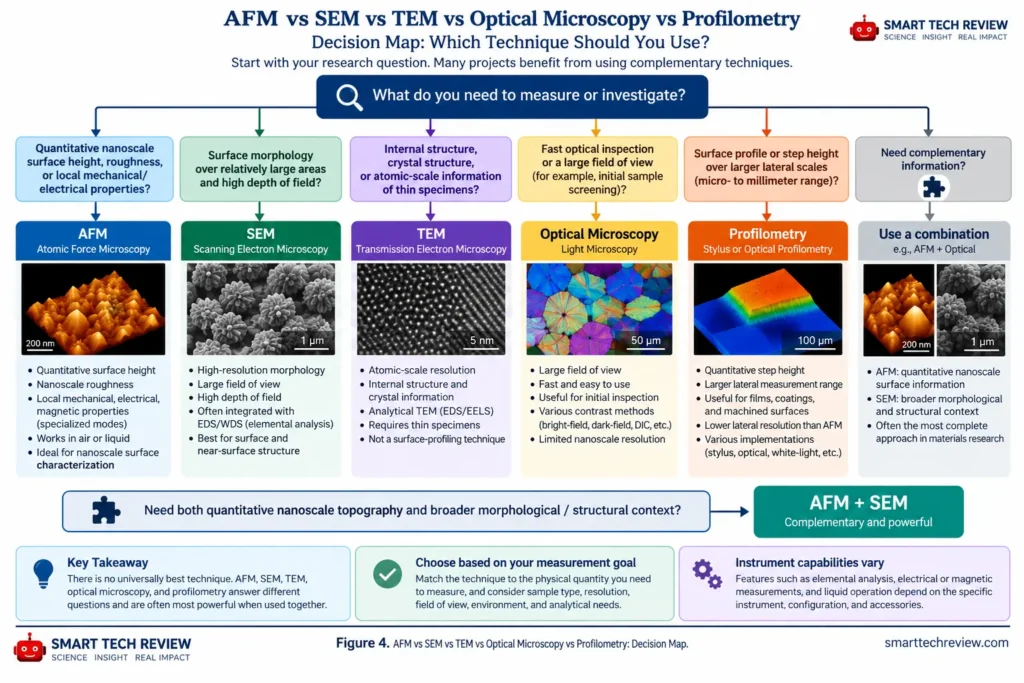
AFM vs SEM: Which Should You Use?

Choose AFM when quantitative surface height, nanoscale roughness, or localized probe-based property measurements are central to the research question.

Choose SEM when rapid visualization of comparatively larger surface areas, high depth-of-field imaging, morphology, or integration with analytical techniques such as EDS is more important.

AFM and SEM therefore should not always be viewed as competing techniques. In many materials-science studies, they provide complementary information:

AFM → quantitative nanoscale surface information
SEM → broader morphological and structural context

For many experiments, the strongest characterization strategy is therefore:

AFM + SEM

What Are the Advantages of AFM?

Atomic force microscopy offers several advantages for nanoscale surface characterization and localized property measurements.

Major advantages include:

• quantitative nanoscale surface-height measurement;
• characterization of both electrically insulating and conducting materials;
• limited sample preparation for many applications;
• operation in air and, with suitable instrumentation, in liquids or controlled environments;
• localized nanoscale measurements;
• multiple specialized methods for mapping mechanical, electrical, electromechanical, and magnetic properties;
• correlation of surface topography with local functional properties.

Unlike techniques that primarily generate image contrast, AFM can provide quantitative height information while also supporting specialized probe-based measurements when the appropriate instrumentation and operating mode are available.

What Are the Limitations of AFM?

AFM also has important limitations that should be considered when designing an experiment or interpreting AFM data.

These include:

• limited scan area compared with many larger-field imaging techniques;
• relatively slow scanning;
• tip-shape and tip-convolution artifacts;
• probe wear and contamination;
• possible deformation or displacement of soft or weakly attached samples;
• sensitivity to vibration, acoustic noise, and other environmental disturbances;
• thermal drift;
• feedback-related artifacts;
• scanner nonlinearities and calibration effects;
• dependence of quantitative results on acquisition and data-processing procedures.

Many of these limitations do not make AFM data unreliable. Instead, they mean that probe condition, instrument calibration, acquisition parameters, environmental control, and data processing must be considered when interpreting the measurement.

Is AFM Nondestructive?

Not universally.

AFM can be nondestructive or minimally perturbative under suitable measurement conditions, but the probe physically interacts with—or responds to forces associated with—the sample surface.

Soft materials, weakly attached particles, fragile nanostructures, and biological specimens may therefore be deformed, displaced, modified, or damaged during measurement if tip–sample interactions are not appropriately controlled.

AFM can be nondestructive or minimally perturbative under appropriate measurement conditions—it is not inherently nondestructive in every experiment.

When Should You Use AFM?

Atomic force microscopy is especially useful when the research question involves:

• nanoscale surface topography;
• quantitative local height or step-height measurements;
• nanoscale surface roughness;
• surface morphology and texture;
• local probe–sample interactions;
• nanoscale mechanical behavior;
• specialized local electrical, electromechanical, or magnetic measurements.

The decision to use AFM should begin with a fundamental experimental question:

What physical quantity do I need to measure?

—not simply:

Which instrument do I have available?

AFM is most valuable when its probe-based measurement principle provides information that directly addresses the research question. In many experiments, it is also most powerful when combined with complementary characterization techniques such as SEM, XRD, Raman spectroscopy, or optical methods.

How Do You Choose the Right AFM?

Choosing the right atomic force microscope requires more than comparing headline specifications.

Important factors include:

• sample type and dimensions;
• required scan range;
• required AFM modes;
• probe compatibility;
• force sensitivity;
• scanner performance and noise;
• closed-loop control;
• thermal drift and stability;
• vibration and environmental control;
• liquid compatibility;
• electrical, electromechanical, or magnetic measurement capabilities;
• automation and throughput;
• software and data-analysis capabilities;
• upgradeability;
• technical support;
• total cost of ownership.

A more useful selection framework is:

Application → Required Measurement → AFM Mode → Probe → Instrument Capability

rather than:

Manufacturer → Model → Specification Sheet

The goal is not simply to choose the AFM with the most impressive specifications, but to choose an instrument configuration capable of making the required measurement reliably on the intended sample.

AFM at a Glance

Question	Short answer
What does AFM stand for?	Atomic force microscopy / atomic force microscope
Technique family	Scanning probe microscopy (SPM)
Core measurement principle	Probe–sample interactions are measured while a probe scans across a surface to reconstruct spatially resolved information
Common outputs	Topography, height, morphology, and roughness
Specialized outputs	Mechanical, electrical, magnetic, electromechanical, frictional, adhesive, and force-related properties
Basic AFM modes	Contact, intermittent-contact/tapping, and non-contact
Can AFM characterize insulating samples?	Yes, conventional topographic AFM does not inherently require a conductive sample
Can AFM operate in liquid?	Yes, with suitable instrumentation and configuration
Does every AFM have atomic resolution?	No
Does every AFM support KPFM, PFM, MFM, or C-AFM?	No
Major interpretation risk	Mistaking measurement artifacts or probe-related effects for real sample features

Frequently Asked Questions About Atomic Force Microscopy

What Does AFM Stand For?

AFM stands for atomic force microscopy when referring to the measurement technique and atomic force microscope when referring to the instrument.

What Does AFM Measure?

Basic AFM primarily provides spatially resolved information about surface topography and height.

Specialized AFM methods can additionally investigate local mechanical, electrical, magnetic, adhesive, frictional, electromechanical, and force-related properties.

The exact quantity being measured depends on the AFM mode, probe, instrument configuration, sample, and experimental conditions.

Can AFM Measure Surface Roughness?

Yes. AFM is widely used to quantify nanoscale surface roughness from topographic height data.

However, reported roughness values can depend on scan size, sampling density, probe geometry and condition, preprocessing, filtering, leveling, artifact correction, and the selected roughness parameter.

For meaningful comparisons, these measurement and processing conditions should be considered alongside the reported roughness value.

Can AFM Achieve Atomic Resolution?

Yes, under particular experimental conditions and with suitable AFM implementations.

Advanced AFM methods have demonstrated atomic-scale and atomic-resolution imaging under carefully controlled conditions.

However, atomic resolution should not be assumed for routine AFM measurements, and the statement that “AFM has atomic resolution” is misleading without specifying the measurement conditions and implementation.

Does AFM Require a Conductive Sample?

No.

Conventional topographic AFM does not inherently require an electrically conductive sample, which allows AFM to characterize many insulating materials without the conductive coatings commonly required for some electron-microscopy workflows.

Specialized electrical AFM methods, however, may require conductive probes, suitable sample configurations, electrical contacts, and additional instrumentation.

Can AFM Work in Liquid?

Yes.

Appropriately configured AFM systems can operate in liquid, making AFM useful for applications involving biological specimens, biomaterials, interfaces, electrochemical systems, and other samples that benefit from liquid environments.

Liquid operation requires suitable probes, fluid cells or sample holders, instrumentation, and measurement conditions.

Does AFM Damage Samples?

It can.

AFM can be minimally perturbative under suitable conditions, but the probe interacts with the sample through physical forces.

The probability of deformation, displacement, or damage depends on factors including sample properties, probe stiffness and geometry, AFM mode, interaction force, adhesion, environment, and scanning conditions.

AFM should therefore not automatically be described as nondestructive.

Is AFM Better Than SEM?

Neither technique is universally better.

AFM is particularly strong for quantitative nanoscale surface height, roughness, and localized probe-based measurements. SEM is particularly powerful for rapid morphological imaging across comparatively larger areas and can be integrated with analytical techniques such as EDS.

In many materials-science experiments, AFM and SEM are complementary rather than competing techniques.

How Accurate Is AFM?

AFM can provide highly accurate quantitative measurements when the instrument is appropriately calibrated and the experiment is properly designed.

However, measurement accuracy and uncertainty can depend on:

• scanner calibration;
• probe geometry and condition;
• detector and scanner noise;
• thermal drift;
• feedback performance;
• environmental stability;
• sample behavior;
• acquisition parameters;
• calibration procedures;
• data-processing methods.

AFM accuracy should therefore be evaluated for the specific measurement and experimental configuration, rather than treated as a universal instrument property.

The Most Important Thing to Understand About AFM

AFM is often introduced as a microscope capable of producing three-dimensional nanoscale images.

That description is useful—but incomplete.

AFM is more accurately understood as a measurement platform that converts controlled probe–sample interactions into spatially resolved information.

That distinction explains why probe selection matters, why lateral dimensions can be distorted by tip geometry, why roughness values depend on measurement and processing conditions, why different AFM modes provide access to different physical properties, and why an advertised instrument resolution does not guarantee the same performance on every sample.

The better experimental question is:

What physical property do I need to measure, what tip–sample interaction contains that information, and what experimental configuration can measure it reliably?

Once that question is answered, AFM becomes much more than an imaging technique.

It becomes a framework for designing nanoscale measurements.

Key Takeaways

• Atomic force microscopy (AFM) is a scanning probe microscopy technique that measures tip–sample interactions while a sharp probe scans across a surface.
• One of AFM’s fundamental strengths is quantitative, spatially resolved surface characterization, particularly topography, morphology, height, and roughness.
• Specialized AFM methods extend the platform to mechanical, electrical, magnetic, electromechanical, frictional, adhesive, and force-related measurements, but these capabilities require appropriate probes, instrumentation, and experimental configurations.
• The three classical AFM interaction regimes are contact, intermittent-contact/tapping, and non-contact AFM.
• AFM resolution is not a single universal specification. It depends on the probe, sample, tip–sample interaction, instrument, environment, feedback, and measurement conditions.
• AFM images should not automatically be interpreted as exact replicas of real surfaces. Tip geometry, probe condition, feedback behavior, drift, scanner behavior, environmental noise, sample deformation, and data processing can influence the measured result.
• AFM is not universally nondestructive, and not every AFM supports every advanced measurement mode.

The most useful framework for planning an AFM experiment is:

Research Question → Property → Tip–Sample Interaction → AFM Mode → Probe → Instrument Capability → Measurement → Interpretation

Core Scientific References

Binnig, G., Quate, C. F., & Gerber, C. (1986). Atomic Force Microscope. Physical Review Letters, 56, 930–933.
DOI: 10.1103/PhysRevLett.56.930

Giessibl, F. J. (2003). Advances in Atomic Force Microscopy. Reviews of Modern Physics, 75, 949–983.
DOI: 10.1103/RevModPhys.75.949

Eaton, P., & West, P. Atomic Force Microscopy. Oxford University Press.

National Institute of Standards and Technology (NIST). Atomic force microscopy and nanoscale dimensional metrology resources.

ISO 19606:2024. Fine ceramics (advanced ceramics, advanced technical ceramics) — Test method for surface roughness of fine ceramic films by atomic force microscopy. The standard addresses AFM surface-roughness measurement within its defined fine-ceramic thin-film scope, including evaluation of probe-tip adequacy for the specified measurements.

Nečas, D., Klapetek, P., and related work. Research on scanning probe microscopy data processing, including leveling, line correction, drift, artifacts, and quantitative surface analysis.

Editorial Note

AFM capabilities vary among instruments, probes, accessories, environments, and operating modes. A capability described in this guide should not be interpreted as being available on every atomic force microscope.

Continue Exploring AFM on Smart Tech Review

Continue with these AFM guides:

How to Choose an AFM

AFM Modes Explained

AFM Resolution Explained

AFM vs SEM

Choosing the Right AFM Mode

Choosing an AFM Probe

Common AFM Artifacts

AFM for Thin Films

AFM for Nanomaterials